1. Overview
A coding agent is a language model wrapped in a harness . On every turn the harness sends the model the task so far and a list of tools. The model answers with a tool call, the harness runs it if permitted, and the output becomes context for the next turn. The most consequential tool is the shell. One Bash call can run tests or rewrite a service, and a user who has turned off per call approval never sees which.
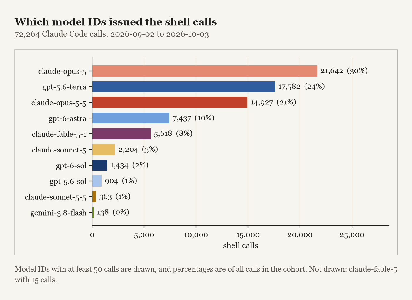
The record so far is short and expensive. In July 2025 a Replit agent reportedly deleted a production database during a code freeze, as logged in the AI Incident Database . In April 2026 Railway described another agent deleting a production volume through its API. In July Hugging Face reported an agent running OpenAI models leaving its evaluation sandbox and reaching five datasets on their infrastructure.
Shell calls are a partial record of that activity, and I wanted a cheap way to say what each one is for. Langfuse’s decision model evaluators can label every call from a fixed list of options at the price of one small model call. What they need is the list itself, with a description and examples for each option. I wanted that list to come from my own traces, not from intuition. So this post embeds and clusters 72,264 recorded Bash calls into a purpose taxonomy, tests how well command text recovers an evaluator’s labels, and compares what four models were given to do. The monitoring signals the taxonomy supports follow, as a design rather than a result, and the remaining observations come last.
The design escalates two kinds of call to an LLM judge or a person. One is labelled other or unclear. The other is labelled differently by the evaluator and a classifier. The review checks each against the session's trajectory for anomalous behavior.
Experimental setup
Grove runs my coding agents in isolated workspaces and acts as their OpenTelemetry gateway. Every observation across every turn of a session leaves as a span. That covers each model request, tool call and result, each annotated with the session, workspace, model, tool name and token counts. Those spans go to whichever OTLP backend is configured, here Langfuse , an open source tracing store for LLM applications. A LiteLLM gateway sits between Claude Code and the providers, so one harness runs Anthropic and OpenAI models interchangeably and the trace records which one answered.
Langfuse runs an evaluator over a filtered set of those observations and stores each answer as a score. An LLM judge would write its verdict in prose. A decision model
, the class TypeSafe
introduced with Jev
, generates no text. It takes the observation as structured state plus a typed question and returns one named option with a probability. Mine is Tev1
, Together AI’s Jev-style 4B fine-tune of Qwen3.5, run as a Q8_0 GGUF on my own GPUs through Ollama’s decision endpoint
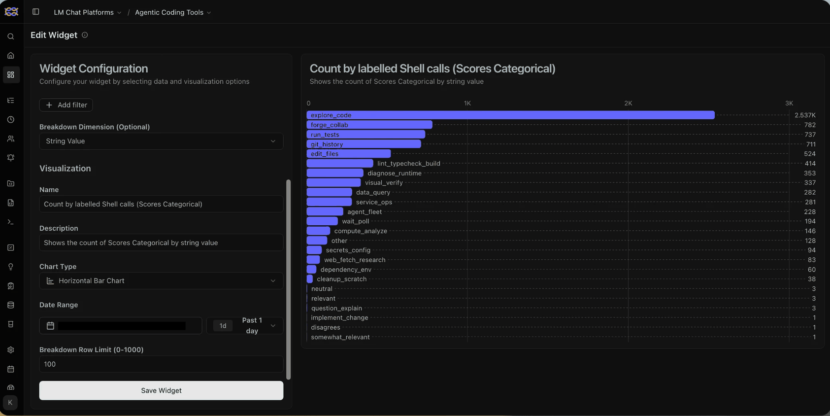
behind the same LiteLLM gateway. Sub second answers at no per call cost are what make labelling every call practical. The question is what is this shell call for, with 18 options such as run_tests. The scores are annotation and never reach the agent.
An illustrative call, not a corpus record:
{
  "type": "tool_use",
  "id": "toolu_example",
  "name": "Bash",
  "input": {
    "command": "uv run pytest tests/test_parser.py -q",
    "description": "Run the parser unit tests"
  }
}
The model generates both command and description before anything runs. One call can hold several shell commands, so call counts are not counts of independent tasks.
Purpose distribution summary
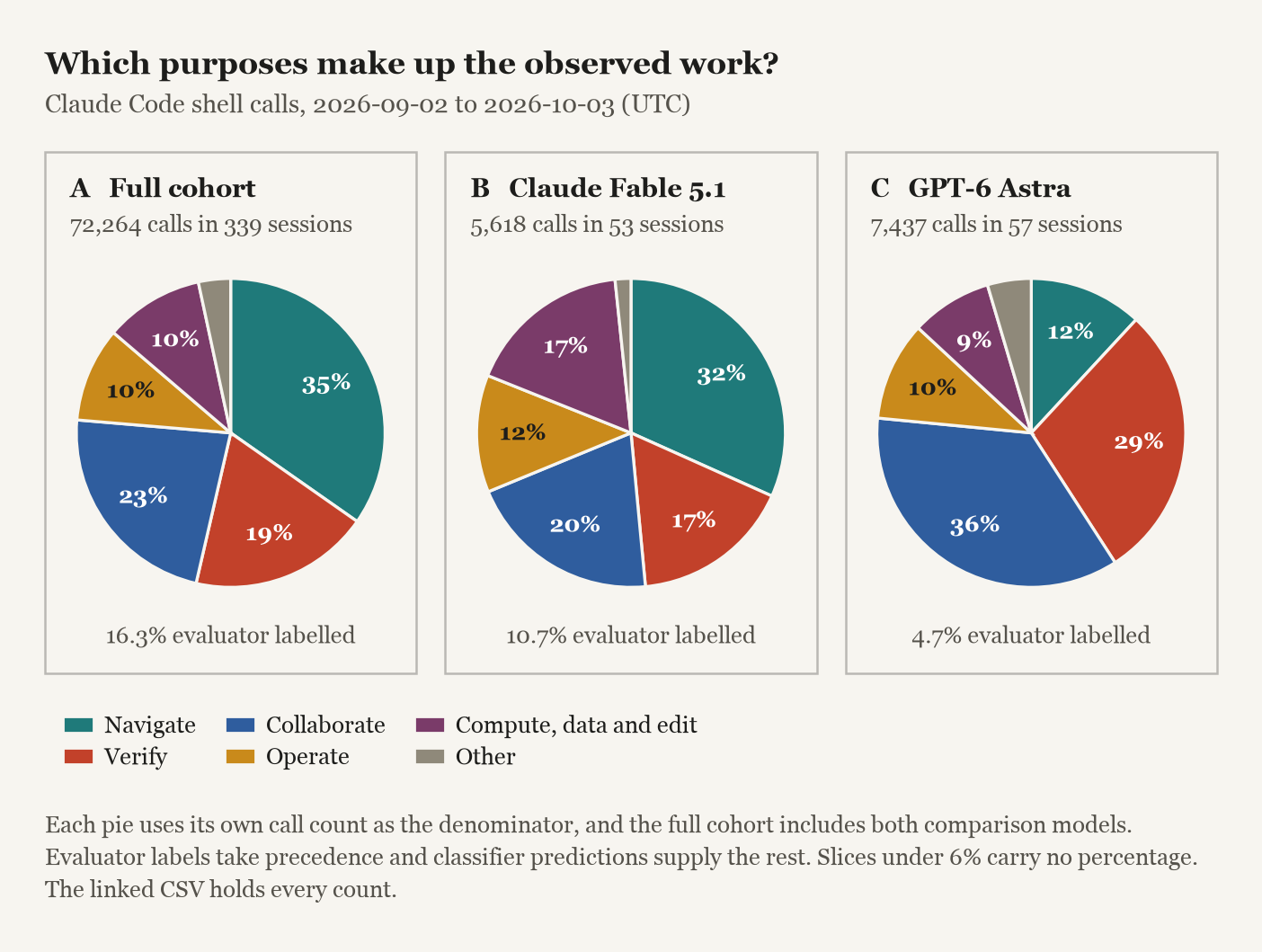
Every call below carries a purpose. The evaluator supplied 16.3% of them and a classifier trained on those labels supplied the rest. No person has checked either. The six broad groups keep every call, clustered or not.
2. Dataset and command embeddings
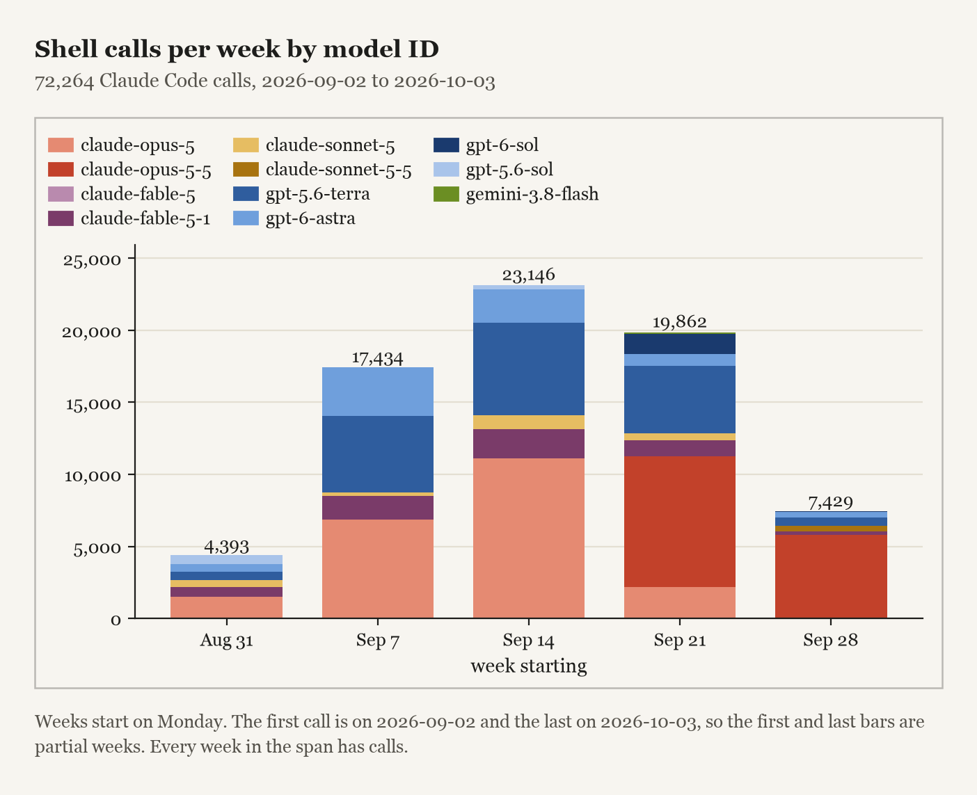
The calls span one month of work. Holding the harness to Claude Code keeps the tool surface constant while models and tasks vary.
| Observation | Selected cohort |
|---|---|
| Claude Code shell calls | 72,264 |
| Recorded session IDs | 339 |
| Calls with an evaluator label | 11,761 |
| Calls assigned a predicted label | 60,503 |
| Sessions containing evaluator labels | 51 |
Qwen3-Embedding-0.6B turns each command into a vector. Long commands are truncated, which can drop the decisive part of a script. The vectors represent the command alone, not the context the model had when it generated it.
3. Predicting evaluator labels
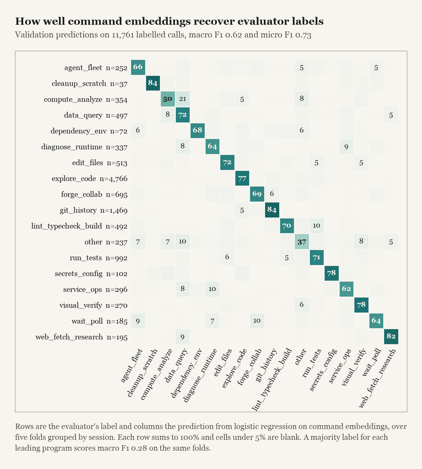
A classifier on command embeddings recovers the evaluator’s labels more than twice as well as the leading program alone. A python3 call might edit a file, query data or run a test, and the program name cannot tell them apart. The full text can.
Logistic regression is trained on the 11,761 labelled vectors, with sessions held apart between training and validation. The table compares it with two baselines.
| Classifier | Macro-F1 | Micro-F1 |
|---|---|---|
| Embedding + logistic regression | 0.62 | 0.73 |
| Embedding + 15 nearest neighbors | 0.52 | 0.72 |
| Leading-program majority | 0.28 | 0.56 |
Macro F1 weights the 18 categories equally and micro F1 pools every decision. The embedding classifier more than doubles macro F1 over the leading program baseline. That is agreement with an LLM judge whose labels no person has validated, not accuracy against ground truth.
4. Clustering and taxonomy derivation
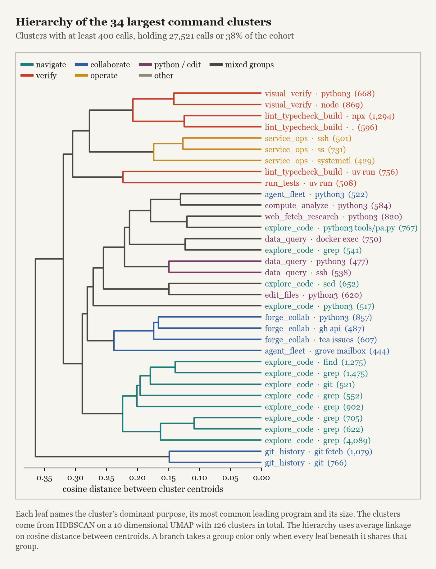
The 18 evaluator labels hide structure that clustering exposes. rg "parse" src/ searches code and sed -n '40,80p' src/parser.py reads a known range, yet both receive the same label. Grouping commands by similarity, without using the labels, separates them.
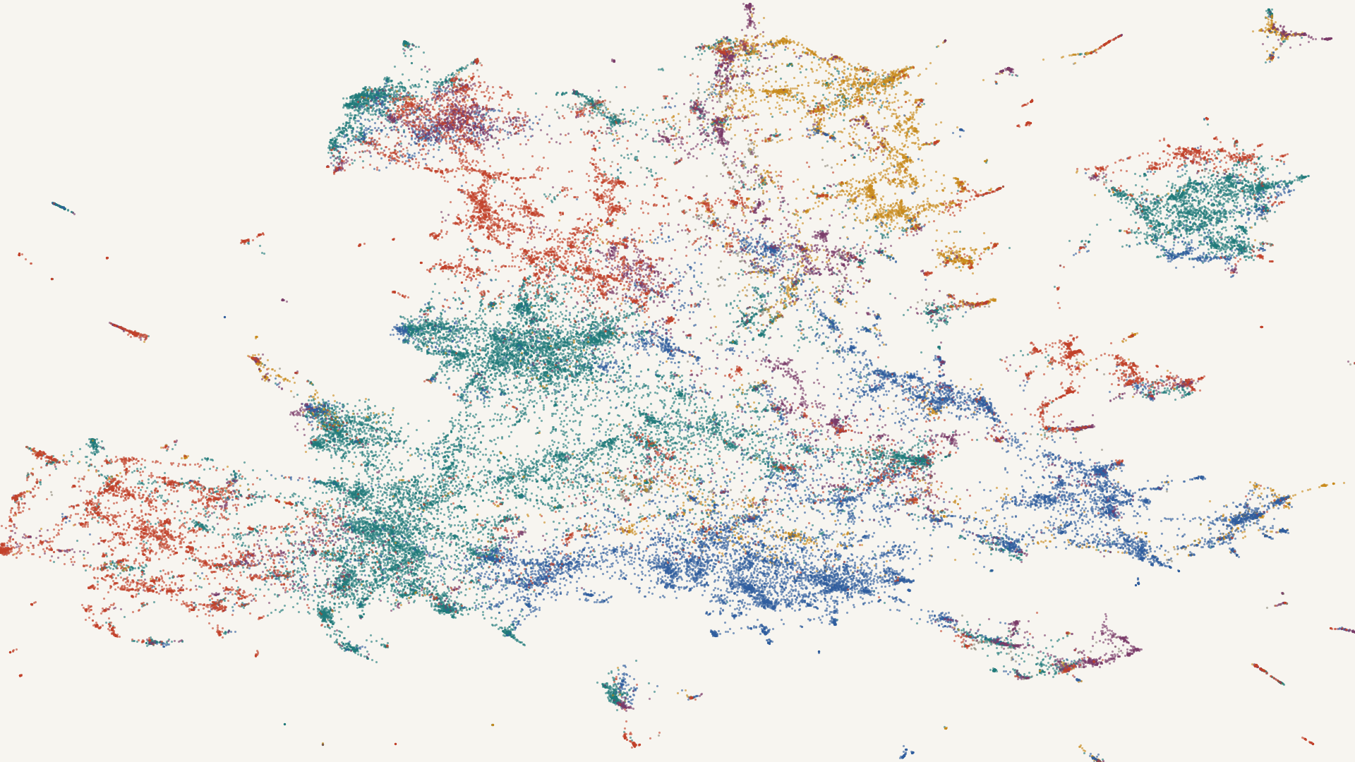
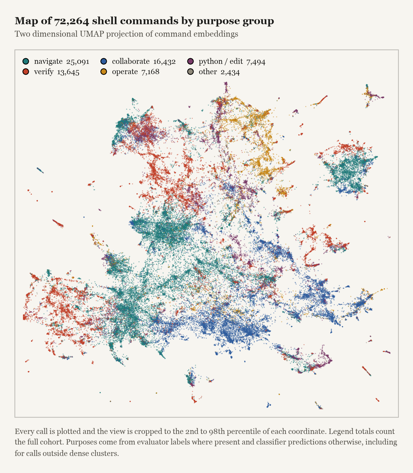
UMAP reduces the vectors to 10 dimensions. HDBSCAN then finds 126 clusters and leaves 33.7% of calls outside any dense group.
On the 8,885 labelled calls inside clusters, agreement with evaluator purposes is modest. The adjusted Rand index is 0.23 and normalized mutual information is 0.35. The clusters do not reproduce the purpose vocabulary, and UMAP can distort density, so they are an inspection aid rather than a validated taxonomy.
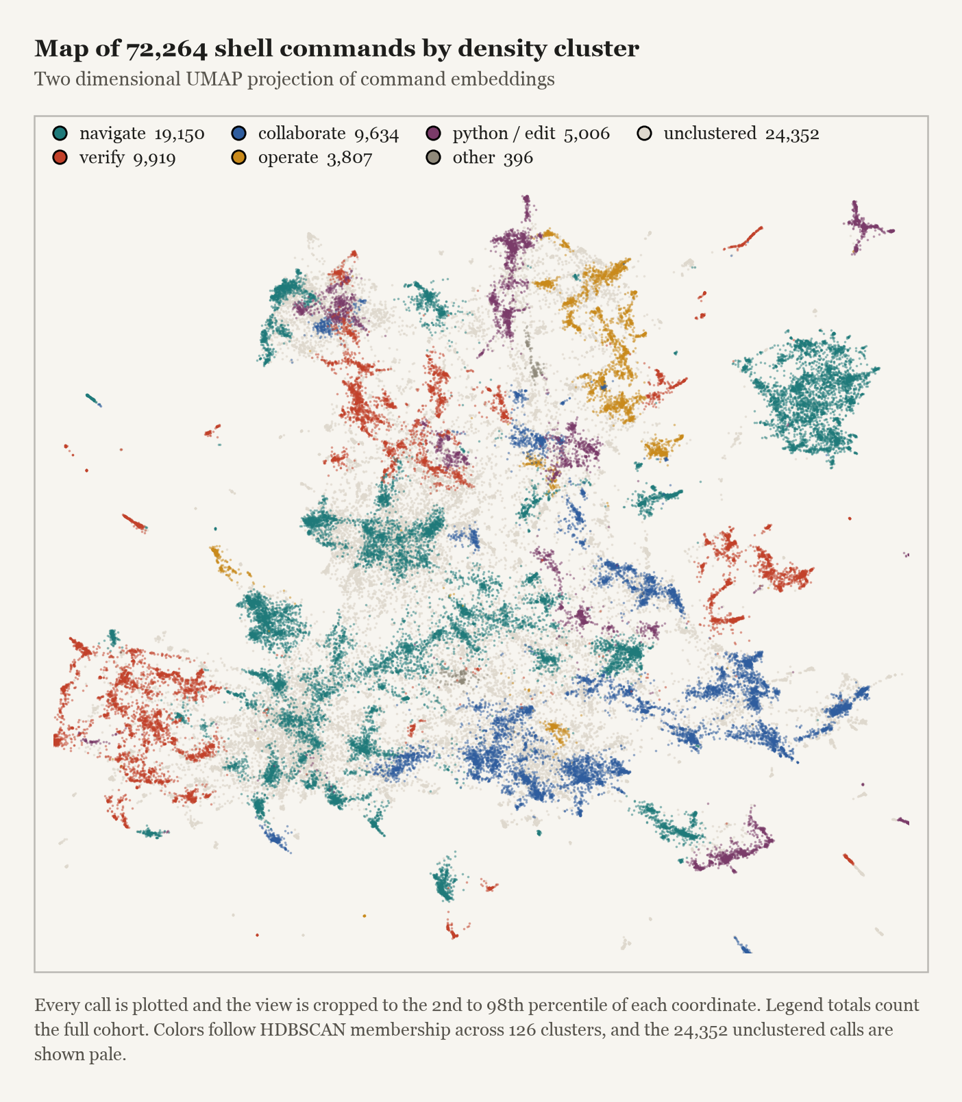
Git history makes up 16.9% of unclustered calls against 10.7% of clustered ones. Dropping the unclustered third would shift the purpose distribution. Every summary keeps every call.
Cluster interpretation and label assignment
The clusters split what one evaluator label merges. Unit tests, browser suites and deliberate mutation checks form separate clusters inside one testing label. Reading code at a past revision separates from searching the current tree. Monitoring CI separates from editing issues and reviews.
I assigned each of the 126 clusters one label by reading its exemplar commands, leading programs and purpose mix. That yields 47 labels in ten families, plus other and unclear as fallbacks. Each unclustered call takes the label of its nearest cluster centroid. That gives every label an approximate share.
Under that approximation 29 labels hold at least 1% of calls, against 16 of the 18 evaluator labels. The largest label falls from 32.7% to 21.2% of calls. No model or person has yet classified individual calls under this taxonomy. These shares describe the clustering, not measured accuracy.
5. Taxonomy adaptation and monitoring design
The Bash call purpose taxonomy
derived above reflects one developer’s workflow. A team can derive its own the same way from its own traces. The evaluator definition
poses it as one choice question with 49 options. Each option carries a description and the clusters behind it. The example command above would map to verify_unit_tests.
The first signal a labelled corpus offers is embedding distance. Cosine distance is one minus cosine similarity. A command far from every validated reference for similar tasks is worth a look. Distance does not establish malice, since commands with similar text can differ in their targets and permissions.
The second is purpose frequency. A team learns the mix of categories its agents normally produce for a kind of task. A run of service_deploy calls during documentation work then stands out. The third is disagreement between the classifier and the evaluator, the fraction of calls they label differently. That measures annotation consistency, not behavior. High disagreement points at an ambiguous category boundary. It should prompt label review, not an alarm.
The disagreeing calls are also the ones to escalate, together with calls labelled other or unclear. Each has a purpose label in doubt. An LLM judge or a person reviews it against the session's trajectory, the task and the turns that led to the call. A command routine in one session can be anomalous in another.
The signals and the escalation path need calibration first. A sample labelled by people would measure accuracy per option and show which clusters need splitting or merging. Alert thresholds would need examples of incidents and of benign activity. I tested neither the signals nor the escalation path, so the monitoring use is a proposed design, not a result.
6. Additional observations
The same corpus also supports comparisons of model exposure, tool errors and associated output tokens, and a separate input comparison measures whether generated descriptions improve purpose classification. None of these feed the taxonomy or the monitoring design. They are reported here because they came out of the labelled data.
Session exposure and purpose distributions
With every call labelled, the purpose mix of each model becomes visible. What it shows is assignment, not ability, and three confounds apply to this subsection and the next. Evaluator coverage varies twelvefold across the four models, from 3.2% to 37.9%. Classifier accuracy was not measured per model, so unequal prediction errors can masquerade as differences in purpose. Attribution names the model that issued a call, not always the one driving the session. And 113 sessions contain more than one model, so the totals are not independent.
A model participates in a session if at least one shell call there is attributed to it. The denominator is all 339 sessions with shell calls.
| Model | Calls | Sessions (% of 339) | Calls/model-session, median (IQR) |
|---|---|---|---|
| Opus 5 | 21,642 | 199 (58.7%) | 55 (14.5 to 142) |
| Opus 5.5 | 14,927 | 101 (29.8%) | 89 (33 to 203) |
| Fable 5.1 | 5,618 | 53 (15.6%) | 44 (16 to 141) |
| GPT-6 Astra | 7,437 | 57 (16.8%) | 86 (34 to 171) |
The two Opus versions never overlap in time, and delegated subagent work is 31.2% of Opus 5 calls against 4.1% for Opus 5.5, so their comparison mixes period with role. Fable’s largest session supplies 16.1% of its calls against 7.6% for Astra. Normalizing by volume does not remove that.
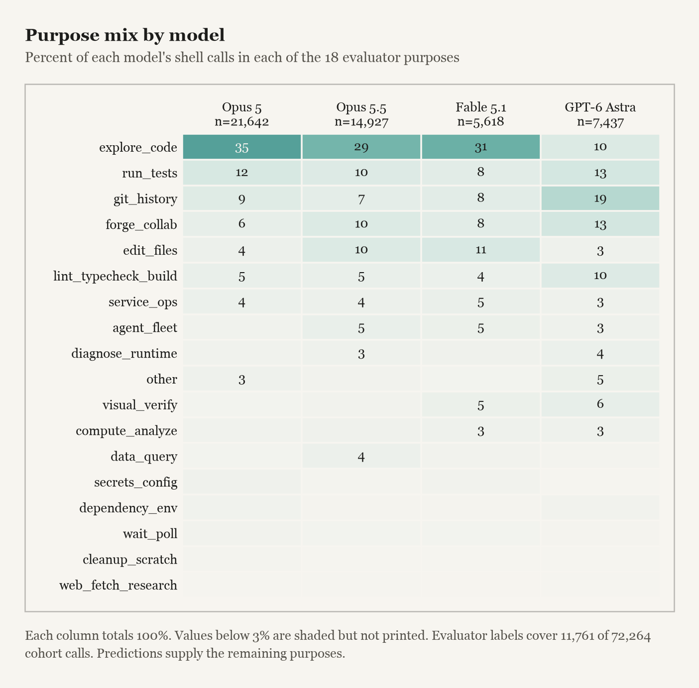
The heatmap weights by calls, so long sessions dominate. Weighting each model and session pair equally gives the shares below.
| Model | Explore code: call → session weighted | Run tests: call → session weighted |
|---|---|---|
| Opus 5 | 34.8% → 30.0% | 12.0% → 8.0% |
| Opus 5.5 | 29.1% → 31.1% | 9.8% → 7.6% |
| Fable 5.1 | 30.7% → 28.1% | 7.7% → 5.3% |
| GPT-6 Astra | 9.9% → 10.7% | 13.1% → 10.2% |
Opus 5 and Opus 5.5 swap order on exploration under session weighting. Astra keeps the lowest exploration share and the highest test share either way.
Tool execution errors
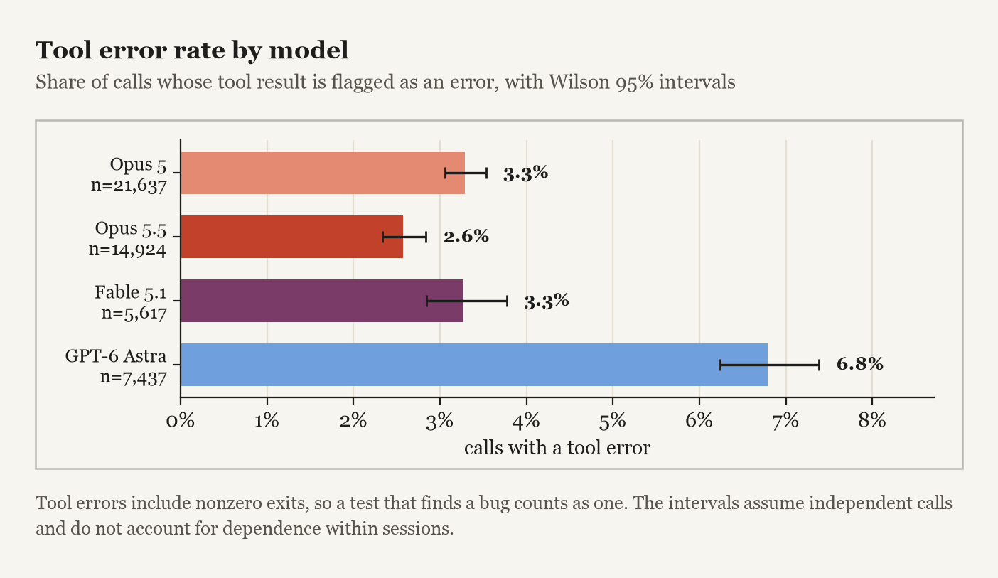
Claude Code’s is_error flag records nonzero exits. A test that finds a bug raises it, so the flag says nothing about whether the task failed. Rates below use only calls that carry the flag.
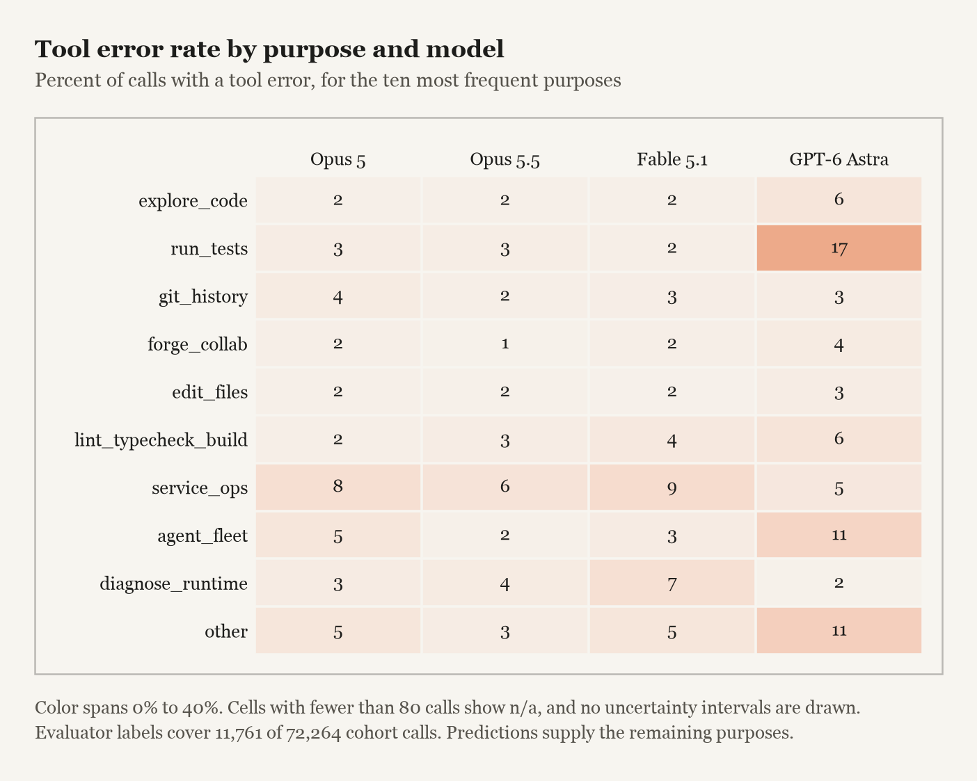
Astra’s aggregate rate is the highest at 6.8%. Yet on service operations Fable errors more often than Astra. Optimizing this flag alone would reward skipping tests over finding and fixing failures. A better outcome would record whether a failing check was resolved and the task accepted.
Command and description features
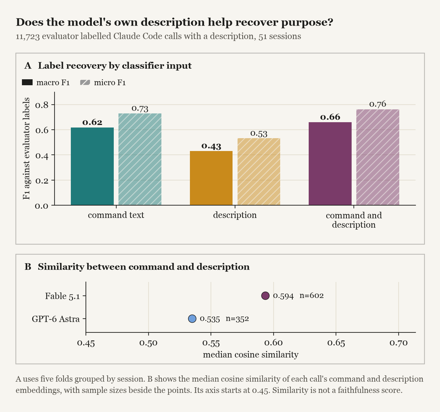
The example above pairs the test command with Run the parser unit tests. On the 11,723 labelled calls that carry a description, I compared classifiers trained on the command, the description and both.
| Classifier input | Macro-F1 | Micro-F1 |
|---|---|---|
| Command | 0.62 | 0.73 |
| Description | 0.43 | 0.53 |
| Command + description | 0.66 | 0.76 |
The description alone is a worse guide than the command. Together they add four points of macro F1, enough to keep the description as a secondary signal. Everything else in this post uses the command classifier alone.
Associated output token distributions
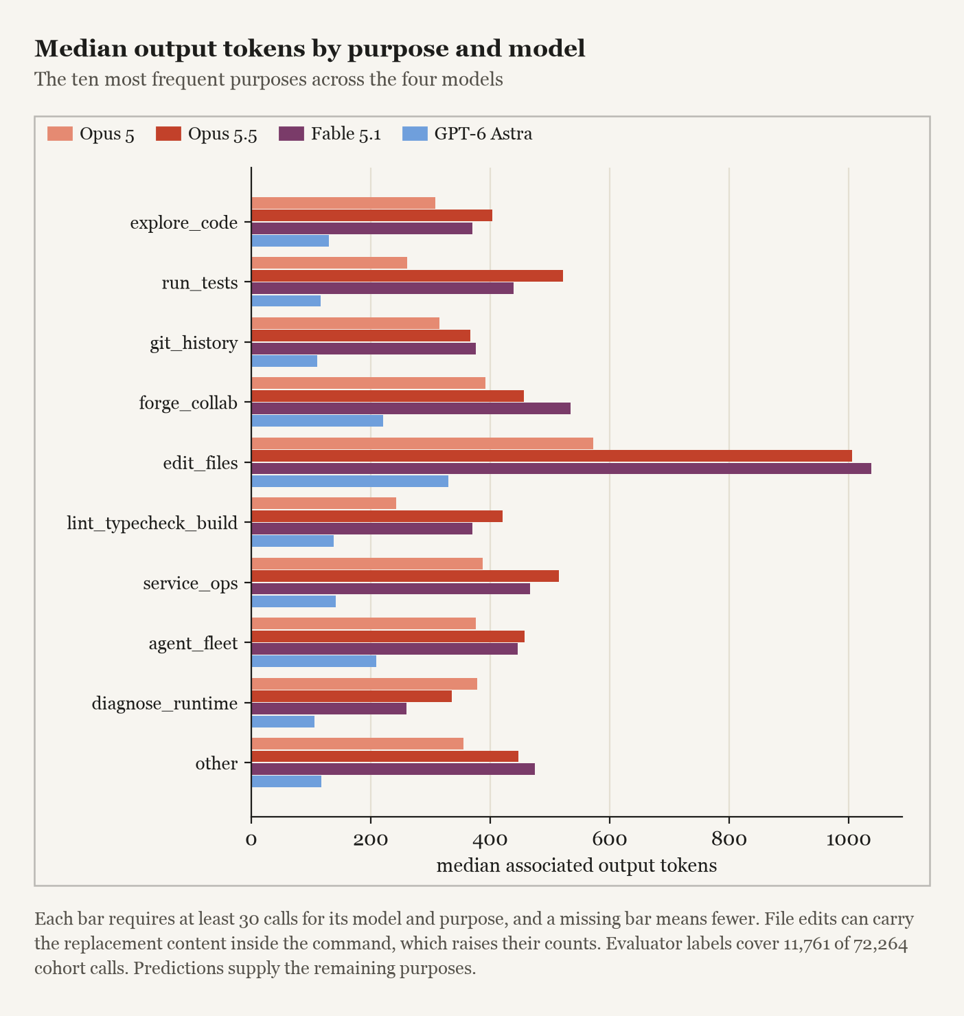
Each call inherits the output token count of the transcript message that issued it. Several calls can share one message. These associated output tokens therefore measure recorded output around shell activity, not a deduplicated bill. Only calls with a positive count enter the comparison.
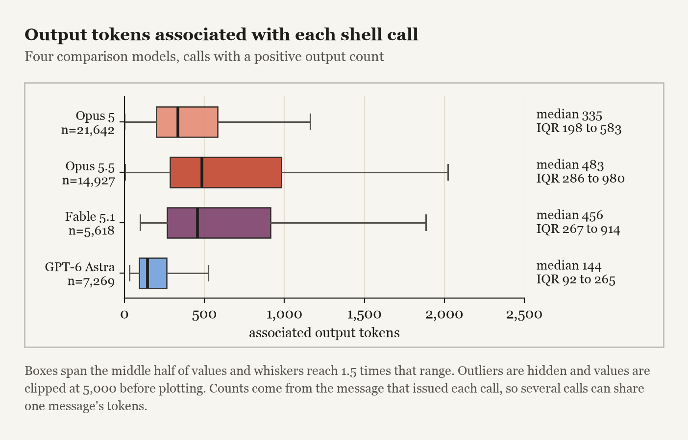
Astra’s median is under a third of the other three. Command payloads and batching count toward these figures alongside any explanatory text.
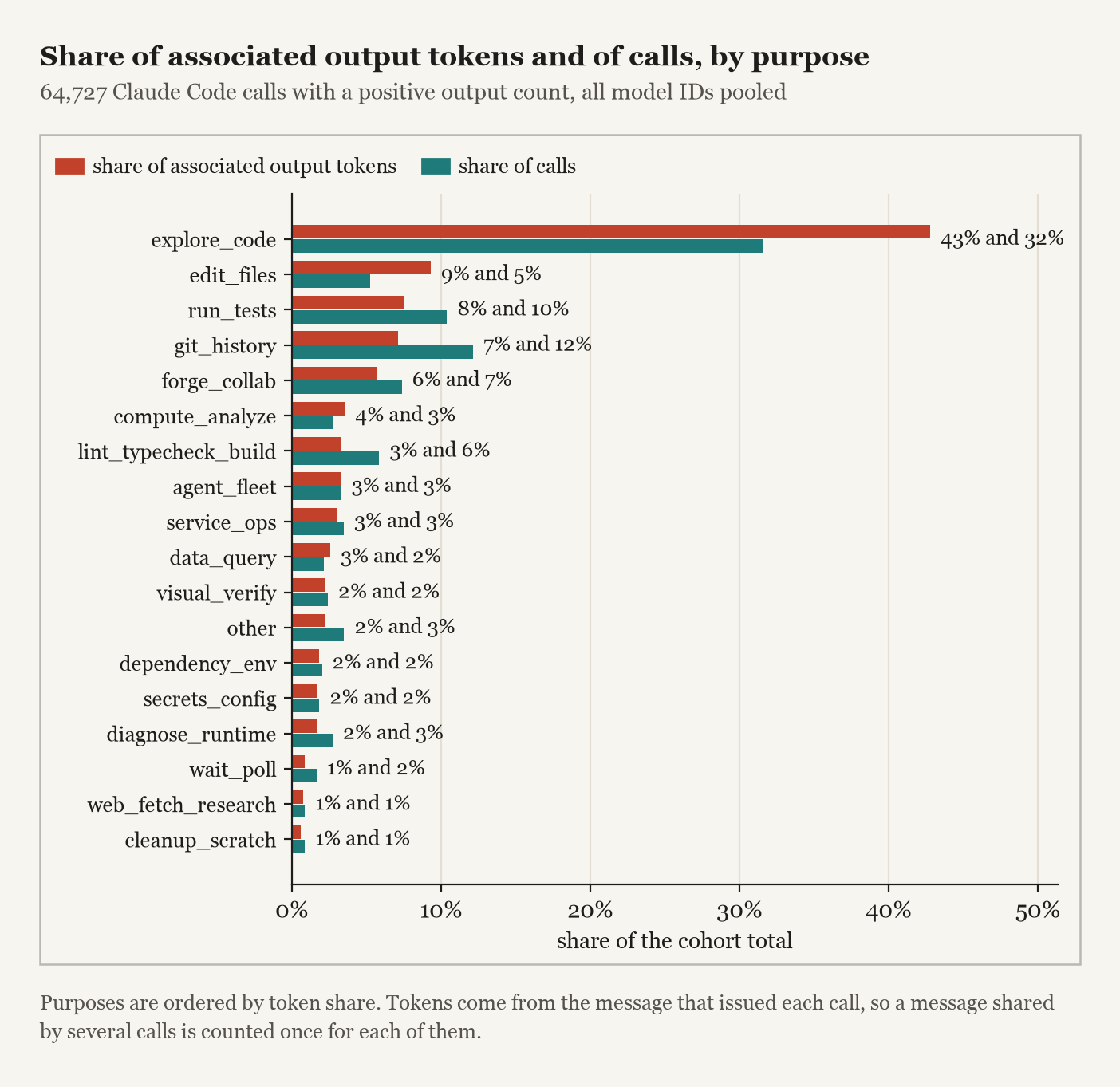
Across the 64,727 eligible calls, exploration is 31.6% of calls and 42.8% of associated tokens. Turning that into savings would need deduplicated messages, input and cache charges, and comparable task outcomes.
Supplementary figures
| Minimum cluster size | Minimum samples | Clusters | Unclustered |
|---|---|---|---|
| 120 | 20 | 126 | 33.7% |
| 120 | 5 | 130 | 31.4% |
| 60 | 20 | 230 | 35.6% |
| 60 | 5 | 266 | 33.0% |
Table S1 compares HDBSCAN settings on the same UMAP coordinates. The unclustered share stays between 31.4% and 35.6% across them.
Reproducibility
Embeddings come from Qwen3-Embedding-0.6B with Q8_0 weights, served through Ollama
, producing 1,024 dimensions. Command text is capped at 2,000 characters, which truncates 2,136 calls or 3.0%. Classification uses logistic regression with five folds from GroupKFold
grouped by session. UMAP uses cosine distance, 30 neighbors and min_dist=0. HDBSCAN uses min_cluster_size=120 and min_samples=20. Other embeddings and UMAP settings were not tested.
Raw traces contain private workspace content and are not released. The CSVs above support inspection of the summaries but cannot reproduce the full analysis.